Creating your own Excel Formulas and doing the impossible


Almost 50 years of programming experience. Click '+ More' in my "Full Biography" to see links to some articles I've written.
Published:
Browse All Articles > Creating your own Excel Formulas and doing the impossible
This article describes how to create your own Excel formula when there isn't a built-in formula that meets your needs.
Create your own formula by
If you are like me then you’ve occasionally found situations where there is no formula (also called a function) in Excel that meets your needs and so you write a macro (or get help writing one) that does the job. That’s good but unless the macro is triggered by some event in Excel like selecting a new cell or selecting a new sheet then you need a manual approach to running it, like a button or a shortcut key. Formulas on the other hand run automatically when the data that they are associated with changes and so it would be nice if you could create your own formula, and as the title of this article says, you can.
The macros mentioned above are a type of Visual Basic for Applications (VBA) code and to create them Excel provides the Visual Basic Integrated Design Environment (the IDE). Two of the main types of code are Subs which don’t return a value when executed and Functions which do, and we are going to use the latter to do what we want.
Fortunately, Excel allows us to write functions that can be used in exactly the same way as the built-in functions. These functions are called User Defined Functions or UDFs. In order to write a UDF you'll need a basic understanding of how to write VBA code. This article will provide some of that information and if you need more then there are several good articles here that will help.
UDFs are created in the IDE and to get there you press Alt+F11. Once there, right-click on your workbook name in the "Project-VBAProject" pane (at the top left corner of the editor window). If you don’t see an existing module, or if you want to add a new one, then select Insert -> Module from the context menu.
To begin, select the module where you want the new UDF to reside.
UDFs like all functions have a name, an argument list, and a return type. Arguments are values passed to the function and with a UDF they are usually ranges. The generic form of a Function declaration is
ScopeKeyword is an optional value that defines the scope of where the function can be used. The allowed values are Public which sets the functions scope to the entire workbook including all the worksheets, and Private which restricts the scope to the module or sheet where the function resides. If the keyword is omitted the function is treated as Public so it's my habit to not include it. FunctionName is the function/formula name, Arg is the first of what could be several arguments, DataType indicates the type of value that the function expects for the argument, and ReturnType indicates the type of value that the function will return. Note that neither DataType nor ReturnType are required, and if left out then Excel will treat them as the Variant data type which will handle all types of data. The problem with Variants is that they are the largest and slowest of the data types but in most cases you won’t notice. My advice however is to use a data type that specifically describes the data like Range or String whenever possible.
For our first UDF let’s assume that you want to add up the absolute values in a range, so that if there were 4 cells in the range and they contained 1, -5, 6 and 8 the result would be 20. I’m certain that a regular formula could be built to do this, but let’s proceed as if it couldn’t.
We’ll call our UDF SumABS and we’ll build it so that it expects one argument of type Range and returns a value of type Double. I could have used one of several other ReturnTypes like Integer or Currency but our UDF might encounter a situation where the sum exceeds the Integer limit of 32,767 and/or it might encounter values with more than Currency's limit of 4 decimal places to the right. Here’s the UDF which once we get by the little bit of math, is pretty simple.
If the values were in cells A1 to A4 then to use the UDF you would enter = SumABS (A1:A4) in a cell or the formula bar.
Note that not only does the ReturnType defines the type of data that the function will return, but it also defines what data type the function is, and since in our case it’s type Double, we don’t need dblTotal and this works just fine.
If you had a situation where you wanted to create a UDF that involved two non-adjacent cells and you knew that, say, the second cell was always 4 cells to the right of the first like with B1 and F1, then you might be tempted to only include a single argument for B1 in the function description and to use .Offset(0, 4) to refer to F1, but that would be a mistake. Writing it that way would work as long as you didn’t just change the value in F1. UDFs only “know” about their arguments so since no argument was provided for F1 the UDF wouldn’t know that F1 had changed, and so the result of the UDF wouldn’t change.
Let’s assume that you need a formula that will return the last row or column of a merged range. Here’s a UDF that I wrote that does just that. Don’t let the ‹ › around the end_col_or_row freak you out – I’ll get to that in a minute.
To use the above as a function, all you need to do is to enter =MergedRange(B7) in the Formula Bar, where B7 is any cell in the merged area. By default the UDF will return the number of the first row, but you could also enter =MergedRange(B7, “endcol”) to get the last column number or =MergedRange(B7, “endrow”) to get the last row number. In a similar fashion the option “col” returns the first column number and “row” returns the first row. Any other optional value returns a #Value! error.
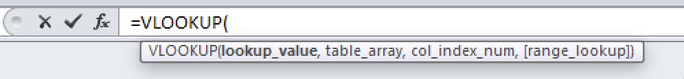
One problem with UDFs is that while when you enter or choose a built-in formula like VLOOKUP and you press the Tab key, IntelliSense shows you this
![Article_Intellisense.jpg]()
which shows the parameters that are expected or optional, but that doesn’t happen with a UDF. The good news is that pressing Ctrl+Shift+A will show you the expected and optional values. There’s still a problem however and that is that if the function header for my UDF was written this way
Then after Ctrl+Shift+A you’d see
![Article_2.jpg]()
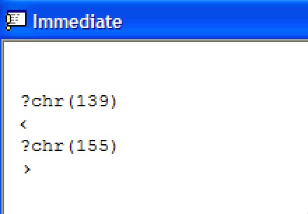
and you wouldn’t know that “end_col_or_row” was optional. You could rename it something like “optional_end_col_or_row” or “opt_end_col_or_row” but it would be nice if we could put square brackets around it. Unfortunately that’s not allowed but you can come close, and that’s because Excel allows you to use any ASCII character between 128 and 255 in a variable name, so in my UDF I added bracket-ish ASCII characters 139 and 155 to the variable name . Note that they are not the same as “<” and “>” which are ASCII 60 and 62. An easy way to generate those "bracket" characters is to type the two lines beginning with "?" into the Immediate Window, press Return, and copy/paste the results into the UDF.
![chr.jpg]() Now Ctrl+Shift+A shows you this
Now Ctrl+Shift+A shows you this
![Article_3.jpg]()
and it’s pretty obvious that it’s optional.
If you’ve seen questions about using a UDF to update two cells you have probably seen the answer as some form of “You can’t do that”. While that’s strictly true, it doesn’t mean it can’t be accomplished with a little bit of code outside the UDF. Consider this problem: You need a formula that will return twice the value of another cell and you also want to place the date of the update in a second cell 6 cells to the right of the first The sticking point is that you don’t know where in the sheet the formula will be used. If you knew the latter piece of information it would be easy to add code in the Worksheet_Change event and use Intersect to determine if the Target cell fell in some range and to update the second cell with today’s date, but since we don’t know the range, what do we do? The following is a solution. (Some clever person may be able to do it some other way, but let’s ignore that.)
In a module add this code:
And in the worksheet where the DoImpossible UDF is going to be used, add this code:
How does it work?
Assume there’s a value of 3 in B10 and we place =DoImpossible(B10) in D10. When you do that the UDF will set D10 to 6 but it will also set gdteUpdateDate to today’s date and set gstrAddressChanged to the address of the cell that was changed. The execution of the UDF causes the worksheet to recalculate and so as long as gstrAddressChanged isn’t blank the date get’s put in the cell six to the right. Tah-Da!
While as with most programming topics there's more to learn about UDFs, I hope that reading this article has given you the information that you need to get started writing your own. If you have any questions that you think are of public interest please post them here. I'd also be happy to answer specific questions sent to me via EE messages.
If you find that this article has been helpful, please click the “thumb’s up” button below. Doing so lets me know what is valuable for EE members and provides direction for future articles. It also provides me with positive feedback in the form of a few points. Thanks!
The basics
The macros mentioned above are a type of Visual Basic for Applications (VBA) code and to create them Excel provides the Visual Basic Integrated Design Environment (the IDE). Two of the main types of code are Subs which don’t return a value when executed and Functions which do, and we are going to use the latter to do what we want.
Fortunately, Excel allows us to write functions that can be used in exactly the same way as the built-in functions. These functions are called User Defined Functions or UDFs. In order to write a UDF you'll need a basic understanding of how to write VBA code. This article will provide some of that information and if you need more then there are several good articles here that will help.
UDFs are created in the IDE and to get there you press Alt+F11. Once there, right-click on your workbook name in the "Project-VBAProject" pane (at the top left corner of the editor window). If you don’t see an existing module, or if you want to add a new one, then select Insert -> Module from the context menu.
Creating a UDF
To begin, select the module where you want the new UDF to reside.
UDFs like all functions have a name, an argument list, and a return type. Arguments are values passed to the function and with a UDF they are usually ranges. The generic form of a Function declaration is
[ScopeKeyword] Function FunctionName (Arg As DataType,……….) As ReturnTypeScopeKeyword is an optional value that defines the scope of where the function can be used. The allowed values are Public which sets the functions scope to the entire workbook including all the worksheets, and Private which restricts the scope to the module or sheet where the function resides. If the keyword is omitted the function is treated as Public so it's my habit to not include it. FunctionName is the function/formula name, Arg is the first of what could be several arguments, DataType indicates the type of value that the function expects for the argument, and ReturnType indicates the type of value that the function will return. Note that neither DataType nor ReturnType are required, and if left out then Excel will treat them as the Variant data type which will handle all types of data. The problem with Variants is that they are the largest and slowest of the data types but in most cases you won’t notice. My advice however is to use a data type that specifically describes the data like Range or String whenever possible.
For our first UDF let’s assume that you want to add up the absolute values in a range, so that if there were 4 cells in the range and they contained 1, -5, 6 and 8 the result would be 20. I’m certain that a regular formula could be built to do this, but let’s proceed as if it couldn’t.
We’ll call our UDF SumABS and we’ll build it so that it expects one argument of type Range and returns a value of type Double. I could have used one of several other ReturnTypes like Integer or Currency but our UDF might encounter a situation where the sum exceeds the Integer limit of 32,767 and/or it might encounter values with more than Currency's limit of 4 decimal places to the right. Here’s the UDF which once we get by the little bit of math, is pretty simple.
Function SumABS(r As Range) As Double
                      Dim cel As Range ' Define a Range variable to be used to
                                       ' step through the cells in the input range
                      Dim dblTotal As Double ' Define a variable to hold the total

                      ' Step through each cell in the range and sum the absolute values
                      For Each cel In r
                          ' Abs is a built-in math function that returns the
                          ' absolute value of a number. The absolute value is
                          ' how far the number is from 0 and since both 5 and -5 are
                          ' 5 away from 0, it gives 5.
                          dblTotal = dblTotal + Abs(cel.Value)
                      Next

                      ' Set the function equal to dblTotal so that it will
                      ' be returned to the sheet.
                      SumABS = dblTotal
End Function.If the values were in cells A1 to A4 then to use the UDF you would enter = SumABS (A1:A4) in a cell or the formula bar.
Note that not only does the ReturnType defines the type of data that the function will return, but it also defines what data type the function is, and since in our case it’s type Double, we don’t need dblTotal and this works just fine.
Function SumABS(r As Range) As Double
                      Dim cel As Range

                      For Each cel In r
                          SumABS = SumABS + Abs(cel.Value)
                      Next

End FunctionA caution about the function arguments
If you had a situation where you wanted to create a UDF that involved two non-adjacent cells and you knew that, say, the second cell was always 4 cells to the right of the first like with B1 and F1, then you might be tempted to only include a single argument for B1 in the function description and to use .Offset(0, 4) to refer to F1, but that would be a mistake. Writing it that way would work as long as you didn’t just change the value in F1. UDFs only “know” about their arguments so since no argument was provided for F1 the UDF wouldn’t know that F1 had changed, and so the result of the UDF wouldn’t change.
A more complex example
Let’s assume that you need a formula that will return the last row or column of a merged range. Here’s a UDF that I wrote that does just that. Don’t let the ‹ › around the end_col_or_row freak you out – I’ll get to that in a minute.
Function MergedRange(merged_range As Range, Optional ‹end_col_or_row› As String = "") As Long
                      Select Case UCase(‹end_col_or_row›)
                          Case "ENDROW"
                              MergedRange = merged_range.MergeArea.Row + merged_range.MergeArea.Rows.Count - 1
                          Case "ENDCOL"
                              MergedRange = merged_range.MergeArea.Column + merged_range.MergeArea.Columns.Count - 1
                          Case "COL"
                              MergedRange = merged_range.MergeArea.Column
                          Case "", "ROW"
                              MergedRange = merged_range.MergeArea.Row
                          Case Else
                              ' Return a #Value! error
                              MergedRange = CVErr(xlErrValue)
                      End Select
End FunctionTo use the above as a function, all you need to do is to enter =MergedRange(B7) in the Formula Bar, where B7 is any cell in the merged area. By default the UDF will return the number of the first row, but you could also enter =MergedRange(B7, “endcol”) to get the last column number or =MergedRange(B7, “endrow”) to get the last row number. In a similar fashion the option “col” returns the first column number and “row” returns the first row. Any other optional value returns a #Value! error.
One problem with UDFs is that while when you enter or choose a built-in formula like VLOOKUP and you press the Tab key, IntelliSense shows you this
which shows the parameters that are expected or optional, but that doesn’t happen with a UDF. The good news is that pressing Ctrl+Shift+A will show you the expected and optional values. There’s still a problem however and that is that if the function header for my UDF was written this way
Function MergedRange(merged_range As Range, Optional end_col_or_row As String = "") As DoubleThen after Ctrl+Shift+A you’d see

and you wouldn’t know that “end_col_or_row” was optional. You could rename it something like “optional_end_col_or_row” or “opt_end_col_or_row” but it would be nice if we could put square brackets around it. Unfortunately that’s not allowed but you can come close, and that’s because Excel allows you to use any ASCII character between 128 and 255 in a variable name, so in my UDF I added bracket-ish ASCII characters 139 and 155 to the variable name . Note that they are not the same as “<” and “>” which are ASCII 60 and 62. An easy way to generate those "bracket" characters is to type the two lines beginning with "?" into the Immediate Window, press Return, and copy/paste the results into the UDF.
 Now Ctrl+Shift+A shows you this

and it’s pretty obvious that it’s optional.
Doing the impossible
If you’ve seen questions about using a UDF to update two cells you have probably seen the answer as some form of “You can’t do that”. While that’s strictly true, it doesn’t mean it can’t be accomplished with a little bit of code outside the UDF. Consider this problem: You need a formula that will return twice the value of another cell and you also want to place the date of the update in a second cell 6 cells to the right of the first The sticking point is that you don’t know where in the sheet the formula will be used. If you knew the latter piece of information it would be easy to add code in the Worksheet_Change event and use Intersect to determine if the Target cell fell in some range and to update the second cell with today’s date, but since we don’t know the range, what do we do? The following is a solution. (Some clever person may be able to do it some other way, but let’s ignore that.)
In a module add this code:
Option Explicit
                      Public gdteUpdateDate As Date
                      Public gstrAddressChanged As String

                      Function DoImpossible(c As Range) As Double
                      DoImpossible = c.Value * 2
                      gdteUpdateDate = Now()
                      gstrAddressChanged = c.Address
End FunctionAnd in the worksheet where the DoImpossible UDF is going to be used, add this code:
Private Sub Worksheet_Calculate()
                          If gstrAddressChanged <> "" Then
                              Range(gstrAddressChanged).Offset(0, 6).Value = gdteUpdateDate
                          End If
                          gstrAddressChanged = ""
End SubHow does it work?
Assume there’s a value of 3 in B10 and we place =DoImpossible(B10) in D10. When you do that the UDF will set D10 to 6 but it will also set gdteUpdateDate to today’s date and set gstrAddressChanged to the address of the cell that was changed. The execution of the UDF causes the worksheet to recalculate and so as long as gstrAddressChanged isn’t blank the date get’s put in the cell six to the right. Tah-Da!
While as with most programming topics there's more to learn about UDFs, I hope that reading this article has given you the information that you need to get started writing your own. If you have any questions that you think are of public interest please post them here. I'd also be happy to answer specific questions sent to me via EE messages.
If you find that this article has been helpful, please click the “thumb’s up” button below. Doing so lets me know what is valuable for EE members and provides direction for future articles. It also provides me with positive feedback in the form of a few points. Thanks!
Almost 50 years of programming experience. Click '+ More' in my "Full Biography" to see links to some articles I've written.
Have a question about something in this article? You can receive help directly from the article author. Sign up for a free trial to get started.
Comments (13)
Author
Commented:Commented:
Author
Commented:Commented:
Here's the nice alternative: a class that suppresses auto-calculation when instantiated and restores the state when destroyed:
Class clsCalcSuppressor
Open in new window
Now all you have to do is include two statements just at the top of any procedure:Open in new window
...and when the procedure ends by any means, the state is restored, because CS is local and therefore gets destroyed.(But what I wonder is: why doesn't the one statement Dim CS As New clsCalculationSuppressor work?)
Of course this technique can be used for many other application properties, e.g., the status bar, displaying alerts, enabling events, the mouse cursor, screen updating...
Commented:
On my part, I have carefully stored the many original Excel user settings using registry entries upon activation (commandar("ply"), decimal seperator, thousand seperator, xlcalculation, ...), modified them for my needs, and then set them back to the original state on the workbook deactivate_event (that is launched on close and opening a workbook in the same excel instance). Curiously, I have noticed that the orginal usersettings remain if if a new Excel instance is created with my workbook previously openned in its own instance. This appears to work alright for my needs at the moment. Tested using Excel 2013 64 bit and Excel 2010 32bit.
As I am a beginner, I suppose the solution you suggested is quicker; I will give it a try once I get a chance. Thanks!
View More